Multi-layer Subsurface Model

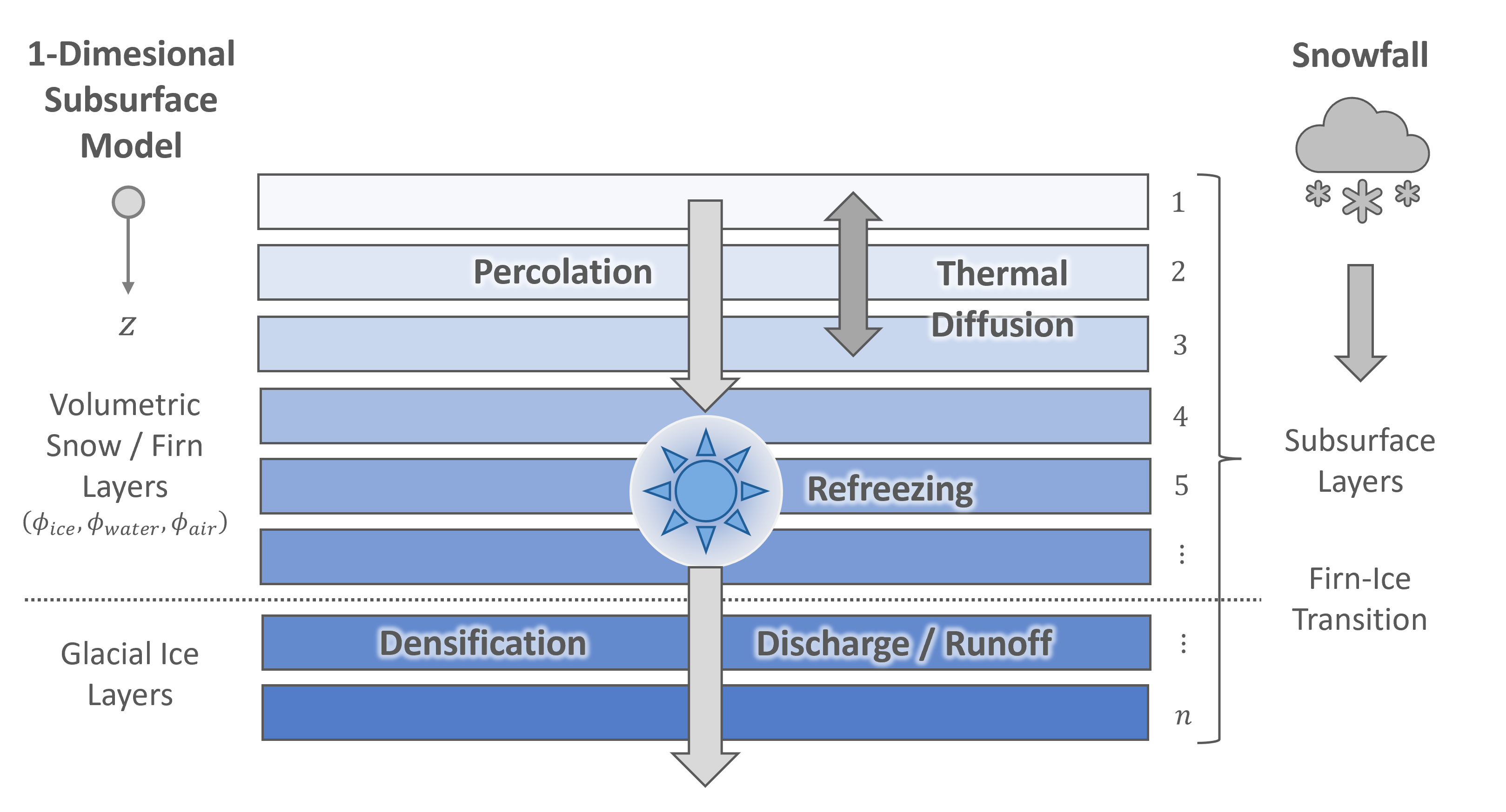
In the FRICOSIPY model, the subsurface is discretised according to an Lagrangian re-meshing algorithm: layers can translate vertically along the depth axis $(z)$ following mass exchange at the surface. Subsurface layers are regulated by a user-defined, fixed height threshold $(h_{\text{max}})$, upon exceeding which a new surface layer is created for further accumulation and all existing layers are shifted downwards.

Subsurface layers are defined according to their volumetric fraction of ice $(\phi_{\text{ ice}})$, water $(\phi_{\text{ water}})$, and air $(\phi_{\text{ air}})$, with most of their inherent physical properties being derived from this volumetric composition.

FRICOSIPY Multi-layer Subsurface Model

Figure 6: FRICOSIPY Multi-layer Subsurface Model

Precipitation

Alt text

Using the standard method, the input precipitation data $(P_{\text{ ref}})$ from the meteorological input file is adjusted to each spatial node $(x,y)$ according to a linear, elevation-dependant precipitation lapse rate $(\Gamma_{\text{ lapse}})$ and a precipitation multiplier $(M)$.

$$ P (x,y) = P_{\text{ ref}} \: \left[\: 1 + (Z (x,y) - Z_{\text{ ref}}) \: \Gamma_{\text{ lapse}} \: \right] \: M $$

where $P_{\text{ ref}}$ and $Z_{\text{ ref}}$ are the reference precipitation data and altitude of the input meteorological dataset, $Z (x,y)$ is the elevation of the spatial node, $\Gamma_{\text{ lapse}}$ is the linear precipitation lapse rate and $M$ is the precipitation multiplier.

Note

It is important to ensure that the reference altitude $(Z_{\text{ ref}})$ of the meteorological station is correctly set for the station_altitude parameter in the parameters.py file.

The FRICOSIPY model then uses a linear logistic transfer function based on the nodal air temperature to differentiate between solid and liquid precipitation. The proportion of snowfall scales between 100 % at 0 °C and 0 % at 2 °C (Hantel et al., 2000). Snow is accumulated into the uppermost subsurface layer; rain is directly routed as liquid into the percolation scheme.

Advanced Precipitation Methods

$(i)$ Mattea et al. (2021)

Alternatively, the user can employ the three-phase anomaly method of Mattea et al. (2021) in which the model temporally downscales a spatially variable annual precipitation climatology into an hourly precipitation time series with adjustments for annual variability.

$$ P (x,y) = C (x,y) \: A(i) \: D (t) $$

where $C$ is the annual precipitation climatology (mm yr$^{-1}$) for a given spatial node $(x,y)$, $A$ is the normalised annual anamoly for a given year $(i)$ and $D$ is the temporal downscaling coefficient for a given timestep (t).

In order to use this method, the following variables must be provided in the input static and meteorological files:

PRECIPITATION_CLIMATOLOGY – Precipitation climatology [m yr$^{-1}$] (input static file)
PRECIPITATION_ANOMALY – Precipitation anomaly [-] (input meteorologicial file)
D – Precipitation downscaling coefficient [-] (input meteorologicial file)

Note

The precipitation anomaly $(A)$ should be expressed as a normalised scaling factor (mean = 1) and the hourly precipitation data should be divided by its annual sum (for each respective year) for the downscaling coefficient $(D)$.

Example

If a person intends to model the Great Aletsch glacier, all meteorological data is available from the Jungfraujoch station (Meteo Swiss), with the exception of precipitation. The user could therefore use the three-phase anomaly method with the following

Precipitation climatology $(C)$ $\rightarrow$ Precipitation 1991-2020 climate normals spatial map
Annual anomaly $(A)$ $\rightarrow$ Monchsgrat annual precipitation measurements
Downscaling coefficient $(D)$ $\rightarrow$ Grindelwald hourly precipitation data

Fresh Snow Density Parameterisations

By default, the density of fresh snow layers $(\rho_{\text{ fresh snow}})$ is defined by the fresh_snow_density parameter. However, the user can also select a more advanced parameterisation to determine a value based on the concurrent meteorological conditions:

$(i)$ Vionnet et al. (2012)

Using the parameterisation of Vionnet et al (2012), the density of fresh snow $(\rho_{\text{ fresh snow}})$ is emperically-derived based on air temperature $(T_a)$ and wind speed $(V)$:

$$ \rho_{\text{ fresh snow}} = \text{max} \left[ \: 109.0 + 6.0 \: T_a + 26.0 \: V^2 , \rho_{\text{ min}} \: \right] $$

where $\rho_{\text{ min}} = 50$ kg m$^{-3}$ is the minimum fresh snow density.

Percolation & Refreezing

Alt text

The FRICOSIPY model employs a standard bucket approach percolation scheme whereby liquid water filters down into subsequent layers upon exceeding the layer saturation capacity – their irreducible water content $(\phi_{\text{ irr}})$.

Penetrating shortwave radiation can also directly melt the ice matrix of subsurface layers, if they are warmed to the melting temperature, supplementing their water content. Subsurface water can also refreeze if there is sufficient cold content and volumetric capacity in layers – the latter being limited by the pore closure density $(\rho_{\text{ pore closure}})$ at the transition from firn to glacial ice.

Advanced Percolation Methods

$(i)$ Darcy (Hirashima et al., 2010)

The parameterisation of Hirashima et al. (2010) simulates the percolation of water through the snowpack based on the Darcy-Buckingham law for fluid flow through an unsaturated porous medium:

\[ q = K \left( \frac{dh}{dz} + 1 \right) \]

where $q$ is the water flux (m s$^{-1}$), $K$ is the hydraulic conductivity (m s$^{-1}$) and $\frac{dh}{dz}$ is the hydraulic suction gradient.

The van Genuchten (1980) model is used to estimate the unsaturated hydraulic conductivity $(K)$ and hydraulic suction head $(h)$ based on a water retention curve for snow:

\[ K = K_\text{ sat} \: \Theta^{\frac{1}{2}} \: \left[\: 1 - \left( 1 - \Theta \right)^m \: \right]^2 \]

\[ h = \frac{1}{\alpha} \: \left( \Theta^{-\frac{1}{m}} - 1 \right)^{\frac{1}{n}} \]

\[ m = 1 - 1/n \]

\[ n = 15.68 \: e^{(-0.46 \: d)} + 1 \]

\[ \alpha = 7.3 \: d + e^{1.9} \]

\[ \Theta = \frac{\theta_{\:w} - \theta_{\:\text{ irr}}}{\theta_{\:ws} - \theta_{\:\text{ irr}}} \]

where $K_\text{ sat}$ is the saturated hydraulic conductivity (m s$^{-1}$), $\Theta$ is the effective water saturation, $d$ is the snow grain size (mm), $\alpha$ & $n$ are the moisture curve characteristic parameters, $\theta_{\:w}$ is the actual volumetric liquid water content, $\theta_{ws}$ is the saturated volumetric water content and $\theta_{\text{ irr}}$ is the irreducible water content.

Typically, the water flux between subsurface layers is then determined by explicitly solving the Darcy-Buckingham equation:

\[ \int_0^{\Delta t} \: q \: dt = K \left( \frac{dh}{dz} + 1 \right) \Delta t \]

However, this explicit scheme quickly becomes numerically unstable for large integration timesteps $(\Delta t)$. Therefore, the water transport model of Hirashima et al. (2010) instead uses a simplified scheme enabling larger timesteps and greater computational efficieny.

\[ \int_0^{\Delta t} \: q \: dt = q_{\text{ lim}} \left[ \: 1 - \text{exp} \left( - \frac{q_0}{q_\text{ lim}} \: \Delta t_{\text{stable}} \: \right) \right] \]

where $q_0$ is the initial water flux and $q_\text{ lim}$ is the limit / maximum amount of water that can be transported in a single stable integration timestep.

The stable integration timestap $(\Delta t_{\text{stable}})$ is determined according to the Courant-Friedrichs-Lewy (CFL) stability condition:

\[ \Delta t_{\text{stable}} \le \frac{1}{2} \text{min} \left( \frac{\Delta z^2}{K \: \frac{dh}{d\theta}} \right) \]

where $\Delta z$ is the layer height (m), $K$ is the hydraulic conductivity (m s$^{-1}$) and $\frac{dh}{d\theta}$ is the inverse moisture gradient (m).

Preferential Percolation Parameterisations

By default, whether using the bucket scheme or Darcy-governed flow, percolation in the FRICOSIPY model adheres to a simple, uniform / homogeneous wetting front. However, in reality, preferential flow can occur where water rapidly penetrates deep into the snowpack in localised columns. This has the potential to advect heat energy to great depths following the latent energy release of refreezing.

$(i)$ Marchenko et al. (2017)

The statistical preferential percolation scheme of Marchenko et al. (2017) initially distributes all surface water in accordance with a normal Probability Density Function (PDF) up to a pre-defined characteristic preferential percolation depth ($z_{\text{lim}}$):

\[ \text{PDF}_{\text{normal}}(z,z_{\text{ lim}}) = 2 \left[ \frac{\text{exp}\left( -\frac{z^2}{2 \sigma^2} \right)}{\sigma \sqrt{2 \pi}} \right] \]

$$ \sigma = z_{\text{ lim}}\: / \: 3 $$

where $\sigma$ is the standard deviation of the probability density function and $z_{\text{ lim}}$ represents the pre-defined characteristic preferential percolation depth (m).

Irreducible Water Content Parameterisations

$(i)$ Coléou and Lesaffre (1998)

Using the parameterisation of Coléou and Lesaffre (1998), the irreducible water content $(\theta_{\text{ irr}})$ is empirically-derived based on observational data.

\[ \theta_{\text{ irr}} = \begin{cases} 9.0264 + 0.0099 \: \frac{(1 \: - \: \phi_{\text{ ice}})}{\phi_{\text{ ice}}},& \phi_{\text{ ice}} \leq 0.23 \\ 0.08 - 0.1023 \: (\phi_{\text{ ice}}-0.03) ,& 0.23 > \phi_{\text{ ice}} \leq 0.812\\ 0 ,& \phi_{\text{ ice}} > 0.812 \end{cases} \]

where $\theta_{\text{ ice}}$ is the volumetric ice fraction of a given subsurface layers.

Saturated Hydraulic Conductivitiy Parameterisations

$(i)$ Shimizu (1970)

Using the parameterisation of Shimizu (1970), the saturated hydraulic conductivity $(K_{\text{ sat}})$ is empirically derived based on laboratory experiments.

$$ K_{\text{ sat}} = 7.7 \times 10^{-4} \: \left[ \: \frac{d^2 g}{\nu} \: \right] \exp \: (-7.8 \times 10^{-3} \: \: \rho) $$

where $d$ is the snow grain size (mm), $g = 9.81$ m s$^{-2}$ is the gravitational acceleration, $\nu = 1.8 \times 10^{-6}$ m$^{-2}$ s$^{-1}$ is the kinematic viscosity of water at 0$^{\circ}$C and $\rho$ is the subsurface layer density (kg m$^{-3}$).

$(ii)$ Calonne et al. (2012)

Using the parameterisation of Calonne et al. (2012), the saturated hydraulic conductivity $(K_{\text{ sat}})$ is empirically-derived based on 3-dimensional image-based computations.

$$ K_{\text{ sat}} = 3.0 \: \left[ \frac{d}{2000} \right]^2 \: \exp \: (-0.0130 \: \rho) \left( \frac{g}{\nu} \right) $$

where $d$ is the snow grain size (mm), $g = 9.81$ m s$^{-2}$ is the gravitational acceleration, $\nu = 1.8 \times 10^{-6}$ m$^{-2}$ s$^{-1}$ is the kinematic viscosity of water at 0$^{\circ}$C and $\rho$ is the subsurface layer density (kg m$^{-3}$).

Note

The parameterisations for hydraulic conductivity $(K_{\text{ sat}})$ are only applicable for users using the Darcy (Hirashima et al., 2010) percolation scheme.

Thermal Diffusion

Alt text

Thermal diffusion, the process by which heat energy moves through the subsurface, is governed by the Fourier heat equation:

$$ \frac{\delta T}{\delta t} = K \: \frac{\delta^{2} T}{\delta z^{2}} = \frac{k}{\rho \: c_p} \: \frac{\delta^{2} T}{\delta z^{2}} $$

where $K$ is the thermal diffusivity (m$^2$ s$^{-1}$), $k$ is the thermal conductivity (W m$^{-1}$ K$^{-1}$), $\rho$ is the density (kg m$^{-3}$) and $c_p$ is the specific heat capacity under constant pressure (J kg$^{-1}$ K$^{-1}$).

In the FRICOSIPY model, the heat equation is numerically solved using an explicit, second-order central difference scheme, constrained between two boundary conditions; the derived surface temperature $(T_{s})$ from the resolution of the surface energy balance (Dirichlet) and a basal / geomethermal heat flux (Neumann).

\[ T_i^{\text{ new}} = T_i + \Delta t_{\text{stable}} \left[ \frac{ \frac{K_{i+1/2}\:(T_{i+1} - T_i)}{\Delta z_{i+1/2}} - \frac{K_{i-1/2}\:(T_i - T_{i-1})}{\Delta z_{i-1/2}} }{ \Delta z_i } \right] \qquad (\text{intermediary nodes}) \]

\[ T_n^{\text{ new}} = T_n + \Delta t_{\text{stable}} \left[ \frac{ \frac{Q_{\text{basal}} K_n}{k_n} - \frac{K_{n-1/2} (T_n - T_{n-1})}{\Delta z_{n-1/2}} }{ \frac{1}{4} z_{n-1} + \frac{3}{4} z_n } \right] \qquad (\text{basal node}) \]

where $i$ is a given subsurface layers, $i \pm 1/2$ represents the interface property between i and the adjacent subsurface layer, $n$ is the total number of subsurface layers, $Q_{\text{ basal}}$ is the basal / geothermal heat flux (W m$^{-2}$) and $\Delta t_{\text{stable}}$ is the stable integration timestep.

The stable integration timestap $(\Delta t_{\text{stable}})$ is determined according to the Von Neumann stability condition:

\[ \Delta t_{\text{stable}} \le \frac{1}{2} \min \left( \frac{\Delta z_{i+1/2}^2}{K_{i+1/2}} \right) \]

Thermal Conductivitiy Parameterisations

$(i)$ Bulk-volumetric

The bulk-volumetric method is the default approach of the original COSIPY model. Thermal conductivity $(k)$ is calculated as a volumetrically-weighted sum of reference values for ice, water and air.

$$ k (\phi) = k_{\:i} \: \phi_{\:i} + k_{\:w} \: \phi_{\:w} + k_{\:a} \: \phi_{\:a} $$

where $k_{\:i}$ = 2.22, $k_{\:w}$ = 0.55 & $k_{\:a}$ = 0.024 W m$^{-1}$ are the reference thermal conductivities and $\phi_{\:i}$,$\phi_{\:w}$ & $\phi_{\:a}$ are the volumetric fractions of ice, water and air respectively.

$(ii)$ Sturm (1997)

Using the parameterisation of Sturm (1997), thermal conductivity $(k)$ is empirically-derived based on observational data.

\[ k (\rho) = 0.138 - 1.01 \: \rho + 3.233 \: \rho^2 \]

where $\rho$ (kg m$^{-3}$) is the density of subsurface layers.

$(iii)$ Calonne et al. (2019)

Using the parameterisation of Calonne et al. (2019), thermal conductivity $(k)$ is empirically-derived based on 3-dimensional image-based computations.

\[ k(\rho,T) = (1-\vartheta) \frac{k_{i}(T) \: k_{\:a}(T)}{k_{\:i}^{\text{ ref}} k_{\:a}^{\text{ ref}}} k_{\text{ snow}}^{\text{ ref}}(\rho) + \vartheta \frac{k_{\:i}(T)}{k_{\:i}^{\text{ ref}}} k_{\text{ firn}}^{\text{ ref}}(\rho) \]

\[ \vartheta = 1 / \left[ 1 + \text{exp}(-2a \: (\rho - \rho_{\:\text{ transition}})) \right] \]

\[ k_{\text{ firn}}^{\text{ ref}} = 2.107 + 0.003618 \: (\rho - \rho_{i}) \]

\[ k_{\text{ snow}}^{\text{ ref}} = 0.024 - 1.23\rho \times 10^{-4} + 2.5 \times 10^{-6}\rho^2 \]

where $k_{\:i}(T)$ and $k_{\:a}(T)$ are the ice and air thermal conductivity at the temperature T, $k_{\:i}^{\text{ ref}}$ = 2.107 and $k_{\:a}^{\text{ ref}}$ = 0.024
W m$^{-1}$ K$^{-1}$ are the ice and air thermal conductivities at the reference temperature of -3 $^\circ$C, $a$ = 0.02 m$^{3}$ kg$^{-1}$ and $\rho_{\:\text{transition}}$ = 450 kg m $^{-3}$.

Specific Heat Capacity Parameterisations

$(i)$ Bulk-volumetric

The bulk-volumetric method is the default approach of the original COSIPY model. Specific heat capacity $(c_p)$ is calculated as a volumetrically-weighted sum of reference values for ice, water and air.

$$ c_p (\phi) = c_{\:p,i} \: \phi_{\:i} + c_{\:p,w} \: \phi_{\:w} + c_{\:p,a} \: \phi_{\:a} $$

where $c_{\:p,i}$ = 2050, $c_{\:p,w}$ = 4217 & $c_{\:p,a}$ = 1004.67 J kg$^{-1}$ K$^{-1}$ are the reference specific heat capacities (for constant pressure) and $\phi_{\:i}$,$\phi_{\:w}$ & $\phi_{\:a}$ are the volumetric fractions of ice, water and air respectively.

$(ii)$ Yen (1981)

Using the parameterisation of Yen (1981), specific heat capacity $(c_p)$ is empirically-derived based on observational data.

$$ c_p (T) = 152.2 + 7.122 \: T $$

where $T$ is the subsurface layer temperature (K).

Firn Densification

Alt text

Firn densification $(\frac{\delta \rho}{\delta t})$ is the process by which snow transforms over time into glacial ice due to overburden pressure and thermal metamorphosis. This excludes the effects of subsurface liquid refreezing, which is already accounted for in the refreezing module.

Firn Densification Parameterisations

$(i)$ Anderson (1976)

The parameterisation of Anderson (1976) is a semi-empirical method that calculates the rate of densification based on the overburden pressure of the snowpack and snow metamorphosis:

\[ \frac{d\rho}{dt} = \left[ \frac{M_s g}{\eta} + c_1 \exp \left[ -c_2 \: (T_m - T_s) - c_3 \max \: (0, \rho - \rho_0 \:) \right] \right] \: \rho \]

\[ \eta \: (z,t) = \eta_0 \:\: \text{exp} \left[ c_4 \: () + c_5 \: \rho \: \right] \]

where $M_s$ is the overlying snow mass, $\eta$ is the snow viscosity (kg m$^{-1}$ s$^{-1}$), $T$ is the current layer temperature (K), $T_m = 273.16$ K is the melting point temperature, $\rho$ is the layer density (kg m$^{-3}$), $c_1 = 2.8 \times 10^{-6}$ s$^{-1}$, $c_2 = 0.042$ K$^{-1}$, $c_3 = .046$ m$^3$ kg$^{-1}$, $c_4 = 0.081$ K$^{-1}$, $c_5 = 0.018$ m$^3$ kg$^{-1}$ and $\eta_0 = 3.7 \times 10^7$kg m$^{-1}$ s$^{-1}$.

$(ii)$ Ligtenberg et al. (2011)

The parameterisation of Ligtenberg et al. (2011) is an enhancement of the semi-empirical method of Arthern et al. (2010), based on the processes of sintering and lattice-diffusion creep of consolidated ice, that adds a dependence on the local accumulation rate $(C)$. It was designed to model firn densification on the Antarctic Ice Sheet (AIS), and is therefore best suited to cold accumulation areas.

\[ \frac{d\rho}{dt} = C \: \: c_{\text{ lig}} \: g \:(\rho - \rho_{\text{ ice}}) \: \text{exp} \left[-\frac{E_{\text{c}}}{RT} + \frac{E_{\text{g}}}{R\overline{T}} \right] \]

$$ c_{\text{lig}}(C, \rho) = \begin{cases} 0.0991 - 0.0103 \: \ln(C), & \rho \lt 550 \text{ kg m}^{-3} \\ 0.0701 - 0.0086 \: \ln(C), & \rho \geq 550 \text{ kg m}^{-3} \end{cases} $$

where $C$ is the accumulation rate (mm yr$^{-1}$), $\rho$ is the layer density (kg m$^{-3}$), $T$ is the current layer temperature (K), $\overline{T}$ is the average layer temperature of the preceding year (K), $R$ = 8.314 J mol$^{-1}$ K$^{-1}$ is the universal gas constant and $E_{\text{c}}$ = 60 kJ mol$^{-1}$ and $E_{\text{g}}$ = 42.4 kJ mol$^{-1}$ are the activation energies associated with creep by lattice diffusion and grain growth respectively.

Note

The FRICOSIPY model determines the accumulation rate ($C$) based on the mean annual mass balance for each spatial node. It is therefore reccomended to precede a simulation using the Ligtenberg et al. (2011) method with a spin-up to enable the simulation to converge on a representative accumulation value. Negative accumulation values (ablation) will simply yield a value of zero for $ln(C)$.

Snow Metamorphism

Alt text

Snow Metamorphism Parameterisations

Snow metamorphosis $(\frac{\delta d}{\delta t})$ is the process by which snow crystals evolve over time, expressed in the FRICOSIPY model by the growth in snow grain size.

$(i)$ Katsushima et al. (2009)

Using the parameterisation of Katsushima et al. (2009), snow grain size $(d)$ growth is determined using the emperical formulations of either Brun (1989) or Tusima (1978); the latter being used when the gravimetric water content is above 10%.

\[ \frac{\delta d}{\delta t} = \begin{cases} \frac{2}{\pi \: d^2} \: \left[ 1.28 \times 10^{-8} + \left( 4.22 \times 10^{-10} \: w^{3} \right) \right], & w \leq 10 \: \% \\ \frac{2.5 \times 10^{-4}}{d^2} \: \frac{1}{3600}, & w > 10 \: \% \end{cases} \]

\[ w = \left[ \frac{\phi_{\:w} \: \rho_{\:w}}{\rho} \right] \]

where $d$ is the snow grain size (mm), $\phi_{\:w}$ is the volumetric liquid water content, $w$ is the gravimetric water content and $\rho_{\:w} = 1000$ kg m$^{-3}$ is the density of water.