Surface Energy Balance

Driven by the input meteorological data, the surface energy fluxes are evaluated at an infinitesimal skin layer to ascertain the surface temperature $(T_s)$. Based on the principles of energy conservation:

$$ SW_{\text{net}} \pm Q_{\text{sensible}} \pm Q_{\text{latent}} \pm LW_{\text{net}} + Q_{\text{rain}} \pm Q_{\text{subsurface}} = 0 $$

where $SW_{\text{net}}$ is the net shortwave radiation flux, $Q_{\text{sensible}}$ and $Q_{\text{latent}}$ are the turbulent fluxes for sensible and latent exchange respectively, $LW_{\text{net}}$ is the net longwave radiation flux, $Q_{\text{rain}}$ is the rain heat flux, and $Q_{\text{subsurface}}$ is the subsurface heat conduction flux (all units W m$^{-2}$).

FRICOSIPY SEB (Surface Energy Balance)

Figure 2: FRICOSIPY Surface Energy Balance

Note

By convention, positive values $(+)$ represent energy absorbed by the glacier surface; negative values $(-)$ depict energy emitted from the glacier surface.

However, since the surface temperature of a glacier is physically constrained to its melting point, excess energy must be apportioned to melt $(Q_{\text{melt}})$ should the surface temperature reach 0 $^\circ$C:

$ \text{if } T_s = 0 \:^\circ\text{C}\: :$

$$ SW_{\text{net}} \pm Q_{\text{sensible}} \pm Q_{\text{latent}} \pm LW_{\text{net}} + Q_{\text{rain}} \pm Q_{\text{subsurface}} = Q_{\text{melt}} $$

The FRICOSIPY model uses an iterative approach to equalise the energy fluxes; the user can select either a Sequential Least SQuares Programming (SLSQP) algorithm or the Newton-Raphson method.

The following section explains each of these energy fluxes in greater detail and how they are parameterised in the FRICOSIPY model.

Shortwave Radiation

Alt text

Shortwave radiation is the thermal radiation supplied directly from the Sun that ranges from the near-ultraviolet (NUV), through the visible light (VIS) and to the near-infrared (NIR) ranges ($\sim$ 0.2 - 3 $\mu$m) of the electromagnetic spectrum. In the FRICOSIPY model, shortwave radiation is modelled after Iqbal (1983) and Klok & Oerlemans (2002):

$$ I_{0} = I_{\text{TOA}} \: \Lambda ( x , y ) \: \tau_{\text{rg}} \: \tau_{\text{w}} \: \tau_{\text{aerosols}} \: \tau_{\text{clouds}} $$

where $I_{0}$ is the solar irradiance, $I_{\text{TOA}}$ is the unattenuated Top-of-Atmosphere (TOA) solar irradiance on a surface normal to the incident radiation, $\Lambda$ is a correction factor for an inclined surface relative to the topography of a spatial node ( $x$ , $y$ ) and $\tau_{\text{rg}}$, $\tau_{\text{w}}$, $\tau_{\text{aerosols}}$ & $\tau_{\text{clouds}}$ are the coefficients of atmospheric transmissivity for Rayleigh scattering and gaseous absorption, water absorption, aerosols and cloud cover respectively .

The coefficients of atmospheric transmissivity that Rayleigh scattering and gaseous absorption $(\tau_{\text{rg}})$, water absorption $(\tau_{\text{w}})$ and the attenuation by aerosols $(\tau_{\text{aerosols}})$ are modelled after Kondratyev (1969), McDonald (1960) and Houghton (1954) respectively. The final component, the attenuation by cloud cover $(\tau_{\text{clouds}})$, is modelled after Gruell et al. (1997):

$$ \tau_{\text{clouds}} = 1 - a \: N - b \: N^2 $$

where $a = 0.233$ and $b = 0.415$ are cloud transmissivity coefficients (default values) and $N$ is the fractional cloud cover.

The incoming shortwave radiation $(SW_{\text{in}})$ is computed as the sum of the direct and diffuse components of the solar irradiance, after Oerlemans (1992); spatial nodes shaded by surrounding topography only receive diffuse radiation.

$$ SW_{\text{in}} = I_{0}\Bigg[ \underbrace{\,0.2 + 0.65(1 - N)\,}_{\text{direct radiation}} \;+\; \underbrace{\,0.8 - 0.65(1 - N)\,}_{\text{diffuse radiation}} \Bigg] $$

where $SW_{in}$ is the incoming shortwave radiation, $I_{0}$ is the solar irradiance and $N$ is the fractional cloud cover.

The net shortwave radiation $(SW_{\text{net}})$ entering the energy balance is calculated using a broadband isotropic albedo $(\alpha)$, that determines the proportion of incoming radiation reflected off the surface. The user can also optionally apportion some of the input shortwave radiation to directly bypass the surface energy balance and directly warm the subsurface layers.

$$ SW_{\text{net}} = SW_{\text{in}} \: (1 - \alpha) - SW_{\text{pen}} $$

where $SW_{\text{net}}$ is the net shortwave radiation, $SW_{\text{in}}$ is the incoming shortwave radiation, $\alpha$ is the broadband albedo and $SW_{\text{pen}}$ is the optional penetrating shortwave radiation deduction.

Albedo Parameterisations

$(i)$ Oerlemans & Knap (1998)

Using the parameterisation of Oerlemans and Knap (1998), the evolution of the broadband albedo
$(\alpha)$ is modelled as an exponentially decreasing function of time $t$ since the last significant snowfall event.

$$ \alpha = \alpha_{\text{firn}} + \left[ (\alpha_{\text{fresh snow}} - \alpha_{\text{firn}}) \: e^{-\frac{t}{t*}} \right] $$

where $\alpha_{\text{fresh snow}} = 0.85$ and $\alpha_{\text{firn}} = 0.52$ are the albedo of fresh snow and firn, respectively (default values),
and $t^*$ is the characteristic decay timescale parameter (days).

$(ii)$ Bougamont et al. (2005)

The parameterisation of Bougamont et al. (2005) is an enhancement of the Oerlemans and Knap (1998) approach. It introduces a surface temperature-dependent albedo decay timescale that enables both a faster decay on a melting surface and slower metamorphism in cold conditions.

\[ t^* = \begin{cases} t^*_{\text{wet}}, & T_s = 0^\circ \text{C} \\ t^*_{\text{dry}} + K \left[ \max(T_s, T_{\text{max}, t^*}) \right], & T_s < 0^\circ \text{C} \end{cases} \]

where $t^∗_{\text{wet}}$ and $t^∗_{\text{dry}}$ are the decay timescales (days) for a melting and dry surface respectively, $K$ is a calibration parameter (day $^\circ$C$^{−1}$) and $T_{\text{max}, t^∗}$ is a temperature threshold ($^\circ$C) for the decay timescale adjustment.

Penetrating Radiation Parameterisation

$(i)$ Bintanja & van den Broeke (1995)

If the user enables the penetrating radiation module, the absorbed radiation $(SW_{\text{pen}})$ at depth $z$ is calculated using the parametersiation of Bintanja and Van den Broeke (1995):

$$ SW_{\text{pen}} (z) = \lambda_{\text{abs}} \: SW_{\text{in}} \: (1 - \alpha) \: e^{-z \: \beta} $$

where $\lambda_{\text{abs}}$ is the fraction of absorbed shortwave radiation ($0.8$ for ice, $0.9$ for snow) and $\beta$ is the extinction coefficient ($2.5$ m$^{-1}$ for ice, $17.1$ m$^{-1}$ for snow as the default values).

Turbulent Fluxes

The turbulent fluxes represent heat and moisture exchange between the atmosphere and the glacier surface, driven by the convective, turbulent motions of the air within the atmospheric boundary layer. In the FRICOSIPY model, the sensible and latent heat fluxes are calculated using bulk aerodynamic equations, which are governed by wind speed, surface roughness, and the gradients of temperature and humidity between the glacier surface and the overlying air.

Note

The magnitude of turbulent exchange heavily depends on the wind speed $(V)$ as strong turbulent motion in the lower atmosphere is needed to maintain strong convective gradients with the surface. In calm conditions / still air, turbulent exchange remains negligible.

Sensible Heat Flux

Alt text

The sensible heat flux represents the transfer of heat energy and is driven by the temperature gradient $(\Delta T)$ between the atmosphere $(T_a)$ and the glacier surface $(T_s)$.

$$ Q_{\text{sensible}} = \rho_{a} \: c_{p,a} \: C_{t} \: V \: (T_{a}-T_{s}) $$

where $\rho_a$ is the dry air density (kg m$^{-3}$), $c_{p,a}$ is the specific heat of dry air under constant pressure (J kg$^{-1}$ K$^{-1}$), $C_{t}$ is the bulk turbulent exchange coefficient, $V$ is the wind speed (m s$^{-1}$), $T$ is the air temperature (K) and the $s$ and $a$ subscripts refer to the surface and the atmosphere at a reference measurement height respectively.

Eg. If the air temperature is warmer than the glacier, sensible / heat energy convects towards and warms the glacier surface.

Latent Heat Flux

Alt text

The latent heat flux represents the transfer of latent energy (associated with phase changes) and is driven by the moisture gradient $(\Delta q)$ between the atmosphere $(q_a)$ and the glacier surface $(q_s)$.

$$ Q_{\text{latent}} = \rho_{a} \: L_{s,v} \: C_{t} \: V \:(q_{a}-q_{s}) $$

where $\rho_a$ is the dry air density (kg m$^{-3}$), $L_{s,v}$ is the latent heat of sublimation or vaporisation (J kg$^{-1}$), $C_{t}$ is the bulk turbulent exchange coefficient, $V$ is the wind speed (m s$^{-1}$), $q$ is the specific humidity (kg kg$^{-1}$) and the $s$ and $a$ subscripts refer to the surface and the atmosphere at a reference measurement height respectively.

Note

The phase change associated with the latent heat flux depends on the glacier surface temperature and the direction of the moisture gradient $(\Delta q)$:

Phase Change	Surface Energy Exchange	Surface Mass Exchange	Surface Temp
Deposition (vapour $\rightarrow$ solid)	Absorption $(+)$	Accumulation $(+)$	$< 0$ $^\circ$C
Condensation (vapour $\rightarrow$ liquid)	Absorption $(+)$	Accumulation $(+)$	$= 0$ $^\circ$C
Evaporation (water $\rightarrow$ vapour)	Emission $(-)$	Ablation $(-)$	$= 0$ $^\circ$C
Sublimation (solid $\rightarrow$ vapour)	Emission $(-)$	Ablation $(-)$	$< 0$ $^\circ$C

Eg. If the surface temperature is less than $0$ $^\circ$C and the air is dry (low specific humidity), sublimation will occur on the surface of the glacier – mass will be lost / ablated as vapour to the atmosphere. The phase transition between a solid and vapour state requires energy and therefore latent energy is drawn / emitted from the surface during this process.

Turbulent Exchange Parameterisation

$(i)$ Essery and Etchevers (2004)

The parameterisation of Essery and Etchevers (2004) defines the bulk turbulent exchange coefficient $(C_{t})$ according to the surface roughness $(\mu)$ and the reference measurement height $(z_a)$:

$$ C_{t} = C_{tn} \: \Psi_{Ri} $$ $$ C_{tn} = \kappa^{2} \left[ \text{log} \left( \frac{z_{a}}{\mu} \right) \right] ^{-2} $$

where $C_{tn}$ is the neutral-condition transfer coefficient, $\kappa = 0.40$ is the von Kármán constant, and $\mu$ is the surface roughness (m).

The stability function $\Psi_{Ri}$, derived from the bulk Richardson number $Ri_b$, corrects for atmospheric stability:

\[ \Psi_{Ri} = \begin{cases} (1 + 10 Ri_{\text{b}})^{-1}, & Ri_{\text{b}} \geq 0 \quad \text{(stable)} \\ 1 - 10 Ri_{\text{b}} \left(1 +10\:C_{\text{hn}} \frac{\sqrt{-Ri_{\text{b}}}}{f_z} \right)^{-1}, & Ri_{b} < 0 \quad \text{(unstable)} \end{cases} \]

\[ Ri_{\text{b}} = \frac{g \: z_\text{a}}{V_{\text{a}}^2} \left[ \frac{T_{\text{a}} - T_{\text{s}}}{T_{\text{a}}} + \frac{q_{\text{a}} - q_{s}}{q_{\text{a}}+\epsilon \: (1-\epsilon)} \right] \]

\[ f_{z} = \frac{1}{4} \sqrt{\frac{\mu}{z_\text{a}}} \]

where $g$ is the gravitational acceleration (m s$^{-2}$) and $\epsilon$ is the ratio of molecular weights between water and dry air.

Surface Roughness Parameterisation

$(i)$ Moelg et al. (2012)

Using the parameterisation of Moelg et al. (2012), the evolution of the surface roughness
$(\mu)$ is modelled as an linearly increasing function of time $t$ since the last significant snowfall event.

$$ \mu = \text{min} \left[ \: \mu_{\text{ fresh snow}} \: t \: t^* , \mu_{\text{ firn}} \: \right] $$

where $\mu_{\text{ fresh snow}} = 0.024$ mm and $\mu_{\text{ firn}} = 4.0$ mm are the albedo of fresh snow and firn, respectively (default values),
and $t^*$ is the characteristic surface roughness timescale parameter (mm h$^{-1}$).

Saturated Vapour Pressure Parameterisations

$(i)$ Sonntag (1994)

Using the parameterisation of Sonntag (1994), the saturated vapour pressure $(VP_{\text{ sat}})$ is empirically-derived based on observational data.

\[ VP_{\text{ sat}} = \begin{cases} a, & T < 0^\circ \text{C} \quad \text{(over water)} \\ a, & T > 0^\circ \text{C} \quad \text{(over ice)} \end{cases} \]

where T is the air of surface temperature ($^\circ \text{C}$).

$(ii)$ Murray (1967) (Magnus-Tetens)

Using the parameterisation of Murray (1967), the saturated vapour pressure $(VP_{\text{ sat}})$ is empirically-derived based on observational data.

\[ VP_{\text{ sat}} = \begin{cases} 6.112 \: \text{exp} \left[ \frac{17.67 \: (T - 273.16)}{T - 29.66} \right] , & T > 0^\circ \text{C} \quad \text{(over water)} \\ 6.112 \: \text{exp} \left[ \frac{22.46 \: (T - 273.16)}{T - 0.55} \right] , & T < 0^\circ \text{C} \quad \text{(over ice)} \end{cases} \]

where T is the air of surface temperature ($^\circ \text{C}$).

Longwave Radiation

Alt text

Longwave radiation (otherwise known as terrestrial radiation) is the thermal radiation emitted between the Earth's surface and atmosphere that is within the infrared classification (3 - 100 $\mu$m) of the electromagnetic spectrum. Net longwave radiation $(LW_{\text{net}})$ is calculated in accordance with the Stefan–Boltzmann law for grey body emission:

$$ LW_{\text{net}} = LW_{\text{in}} - \varepsilon_{s} \: \sigma \: T_{s}^{4} $$

where $LW_{\text{net}}$ is the net longwave radiation flux, $LW_{\text{in}}$ is the incoming longwave radiation, $\varepsilon_{s} \approx 0.99$ is the surface emissivity, $\sigma = 5.67 \times 10^{-11}$ W m$^{-2}$ K$^{-4}$ is the Stefan-Boltzmann constant and $T_s$ is the surface temperature (K).

Longwave Radiation Parameterisation

$(i)$ Konzelmann et al. (1994)

If the user is unable to provide incoming longwave radiation $(LW_{\text{in}})$ in the input meterological data, it can instead by derived from the fractional cloud cover $(N)$ using the parametersiation of Konzelmann et al. (1994). This substitutes the air temperature $(T_a)$ and atmospheric emissivity
$(\varepsilon_{atm})$ into the Stefan-Boltzmann law:

$$ LW_{\text{in}} = \varepsilon_{\text{atm}} \: \sigma \: T_{a}^{4} $$ $$
\varepsilon_{atm} = \varepsilon_{\text{cs}} \: ( 1 - N^2) + \varepsilon_{\text{clouds}} \: N^2 $$
$$ \varepsilon_{cs} = 0.23 + c_{\text{emission}} \left[ \frac{VP_{\text{sat}} \: RH}{T_a} \right] $$

where $LW_{in}$ is the derived incoming longwave radiation, $\varepsilon_{\text{atm}}$, $\varepsilon_{\text{cs}}$ and $\varepsilon_{\text{clouds}} = 0.96$ are the atmospheric, clear-sky and cloud emissivities respectively, $N$ is the fractional cloud cover, $RH$ is the relative humidity (%), $VP_{\text{sat}}$ is the saturated vapour pressure (Pa), $T_a$ is the air temperature (K) and $c_{\text{emission}} = 0.4$ is a calibration parameter.

Rain Heat Flux

Alt text

The rain heat flux represents the energy imparted to the surface from the enthalpy of rainfall:

$$ Q_{\text{rain}} = \rho_{w} \: c_{p,w} \: dt \: (T_{a}-T_{s}) $$

where $\rho_{w}$ is the density of water (kg m$^{-3}$), $c_{p,w}$ is the specific heat of water under constant pressure (J kg$^{-1}$ K$^{-1}$), $dt$ is the model time step and the $T_{s}$ and $T_{a}$ are the surface and air (rain) temperature respectively.

Note

Typically the rain heat flux does not contribute significantly to the surface energy balance; however, the subsequent refreezing of percolating rainwater can greatly influence the thermal state of the subsurface through the release of latent energy.

Subsurface Heat Flux

The subsurface heat conduction flux (otherwise known as the ground heat flux) is determined based on the near surface temperature gradient $(\frac{\delta T}{\delta z})$:

$$ Q_{\text{subsurface}} = k_{s} \: \frac{\delta T}{\delta z} \approx k_{s} \: \left[ \frac{T_{z\:\text{interp 2}} - T_{z\:\text{interp 1}}}{z_{\:\text{interp 2}} - z_{\:\text{interp 1}}} \right] $$

where $k_{s}$ is the surface thermal conductivity (W m$^{-1}$ K$^{-1}$) and $z_{\:\text{interp 1}} = 0.06$ m and $z_{\:\text{interp 2}} = 0.10$ m are the default prescribed depth values used to calculate subsurface temperatures via linear interpolation between subsurface layers.

Melt Energy Flux

Alt text

When the surface temperature $(T_s)$ is evaluated to 0 $^\circ$C, the residual energy $(Q_{\text{melt}})$ melts the glacier surface – the uppermost subsurface layer of the model. This surface melt, combined with any rain or condensation, is then transferred into the percolation routine of the subsurface model where it is stored as liquid water in the snow/firn layers, refreezes (if there is sufficient cold content) or becomes run-off.

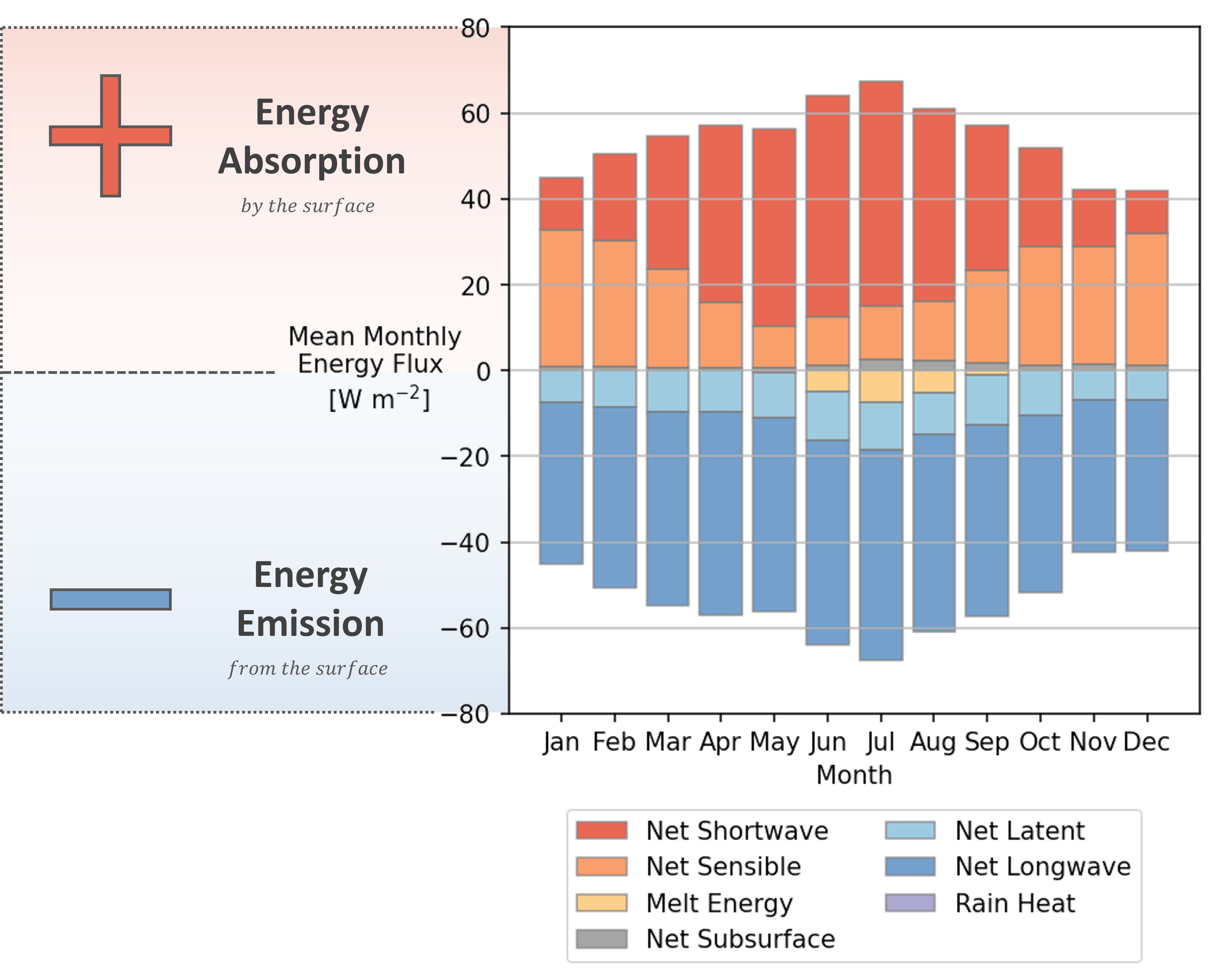
Exemplar Surface Energy Balance

Visualising the Surface Energy Balance (SEB) is important for understanding and analysing the energy exchanges occuring at the glacier surface. According to the priniciples of energy conservation, the opposing monthly energy fluxes must always be balanced. Figure 3 shows an exemplar point surface energy balance for Colle Gnifetti at the summit of the Grenz glacier, Valais, Switzerland produced from the FRICOSIPY model. For Colle Gnifetti, being a high-altitude, wind-exposed glacierised saddle, turbulent exchange has a significant contribution to energy turnover and melt is minimal and confined to the summer months.

Exemplar FRICOSIPY SEB (Surface Energy Balance) Colle Gnifetti

Figure 3: Exemplar point Surface Energy Balance (SEB) for Colle Gnifetti (Grenz glacier), Valais, Switzerland

Note

The FRICOSIPY result viewer contains a plotting function that can automatically produce a surface energy balance graph (akin to the figure above) for any output dataset.

Phase Change	Surface Energy Exchange	Surface Mass Exchange	Surface Temp
Deposition (vapour \(\rightarrow\) solid)	Absorption \((+)\)	Accumulation \((+)\)	\(< 0\) \(^\circ\)C
Condensation (vapour \(\rightarrow\) liquid)	Absorption \((+)\)	Accumulation \((+)\)	\(= 0\) \(^\circ\)C
Evaporation (water \(\rightarrow\) vapour)	Emission \((-)\)	Ablation \((-)\)	\(= 0\) \(^\circ\)C
Sublimation (solid \(\rightarrow\) vapour)	Emission \((-)\)	Ablation \((-)\)	\(< 0\) \(^\circ\)C